Bivariate Kernel Density Estimation Demonstration
Several examples show how to use the gkdeb2 function.
Contents
- Distribution with unbounded support
- Distribution with upper and lower bounds: uniform distribution
- Distribution with lower bound only: exponential distribution
- Distribution with lower bound only: log-normal distribution
- Distribution with lower bound only: chi-square distribution
- Distribution with lower bound only: Rayleigh distribution
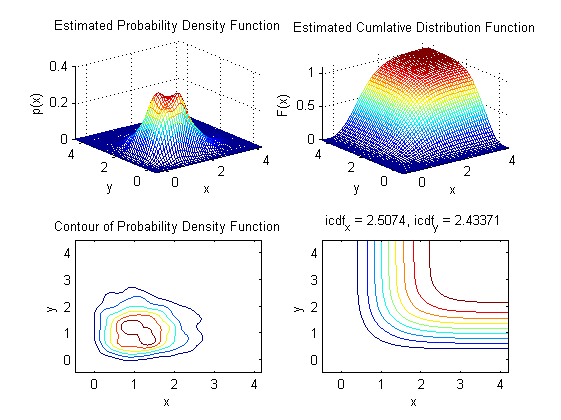
Distribution with unbounded support
Distribution with four peaks.
x = [randn(100,1), (randn(100,1)-10)*2;
      randn(100,1)+10, randn(100,1);
      randn(100,1)+10, (randn(100,1)-10)*2;
      randn(100,2)];
gkde2(x);

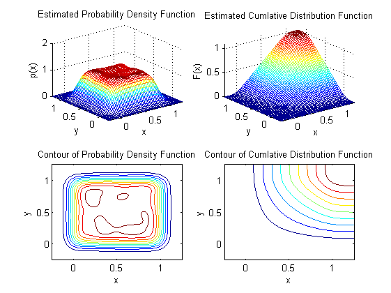
Distribution with upper and lower bounds: uniform distribution
clear
x=rand(10000,2);
% PDF with bounded support
p.xylim=[0 0 1 1];
gkde2(x,p);
% Compare with unbounded PDF estimate
figure;
gkde2(x);


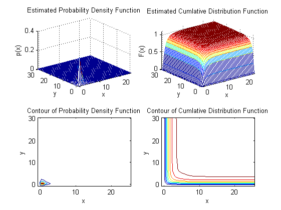
Distribution with lower bound only: exponential distribution
clear
x=-log(rand(1000,2));
% PDF with bounded support
p.xylim=[0 0 Inf Inf];
gkde2(x,p);
% Compare with unbounded PDF estimate
figure
gkde2(x);


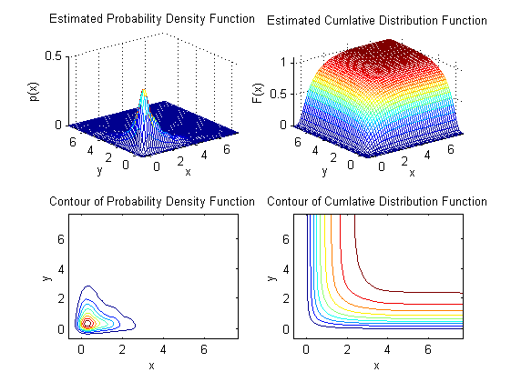
Distribution with lower bound only: log-normal distribution
clear
x=exp(randn(1000,2));
% PDF with bounded support
p.xylim=[0 0 Inf Inf];
gkde2(x,p);
% Compare with unbounded PDF estimate
figure
gkde2(x);


Distribution with lower bound only: chi-square distribution
clear
x=randn(1000,2).^2;
% PDF with bounded support
p.xylim=[0 0 Inf Inf];
p.alpha=0.95;
gkde2(x,p);
% Compare with unbounded PDF estimate
figure
p1.alpha=0.95;
gkde2(x,p1);


Distribution with lower bound only: Rayleigh distribution
clear
x=sqrt(randn(2,1000).^2 + randn(2,1000).^2);
% PDF with bounded support
p.xylim=[0 0 Inf Inf];
p.alpha=0.95;
gkde2(x,p);
% Compare with unbounded PDF estimate
figure
p1.alpha=0.95;
gkde2(x,p1);

