Constrained Total Variation Projection with ADDM

Test for ADMM algorithm convergence on a randomized example.

addpath('../');
addpath('../toolbox/');

We want to solve a problem of the form

 |min_{x in C, norm(K*x,1)<=1} -<x,w> + epsilon/2*norm(x)^2

Here K is some sort of "gradient" operator (here we use a random matrix) and C

This can be written as

 |min_x F(K*x) + G(x)|

where F(u) = i_{norm(u,1)<=1} and G(x) = i_{C}(x) - f,w + epsilon/2*norm(f)^2.

Inner product shortcut.

dotp = @(u,v)sum(u(:).*v(:));

Dimension of the problem.

n = 300;

Number of computed "gradient".

p = 500;

Number of affine constraint

r = 10;

Regularization.

epsilon = .1;

Gradient operator.

K = randn(p,n);

Linear function to optimize.

w = randn(n,1);

Constraint operator.

A = randn(r,n);
y = randn(r,1)*0;

Projector on A*f=y.

pA = A'*(A*A')^(-1);
ProjC = @(f)f + pA*(y-A*f);

Projection on L1 ball.

ProxF = @(u,rho)perform_l1ball_projection(u,1);
ProxFS = compute_dual_prox(ProxF);

Proximal operator of G.

ProxG = @(x,tau)ProjC( (x+tau*w)/(1+tau*epsilon) );

Callback to record information during the iterations.

F = @(x)-dotp(x,w) + epsilon/2*norm(x(:))^2;
Constr = @(x)norm(K*x,1);
options.report = @(x)struct('F', F(x), 'Constr', Constr(x));

Run the algorihtm.

options.niter = 5000;
[f,R] = perform_admm(zeros(n,1), K, K', ProxFS, ProxG, options);

[********************]

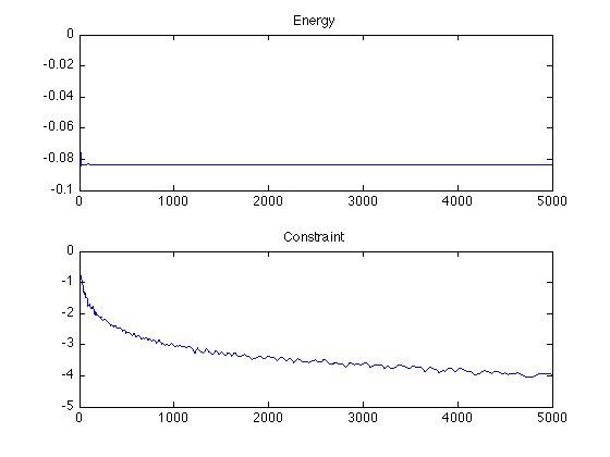
Retrieve the F and constraint function values.

f = s2v(R,'F');
constr = s2v(R,'Constr');

Display.

clf;
subplot(2,1,1);
plot(f);
title('Energy');
subplot(2,1,2);
plot(log10(abs(constr-1)));
title('Constraint');