Brick Highlights

You will find below demos for a few Brick functions, from basic operations to GUI programs. There are many more to discover in the Function Reference !

Contents

Basic operations

fn_coerce is a shortcut for min(max(x,m),M)

Array manipulations

fn_add and fn_mult can add (or multiply) together two arrays which are not the same size, provided that for any dimension where the size differs, this size is 1 for one of the two arrays. The functions guess how to use repmat and make the two inputs the same size.

fn_add(10:10:40,(1:3)')

ans =

    11    21    31    41
    12    22    32    42
    13    23    33    43

fn_mult(ans,[.01 .1 1 10])

ans =

    0.1100    2.1000   31.0000  410.0000
    0.1200    2.2000   32.0000  420.0000
    0.1300    2.3000   33.0000  430.0000

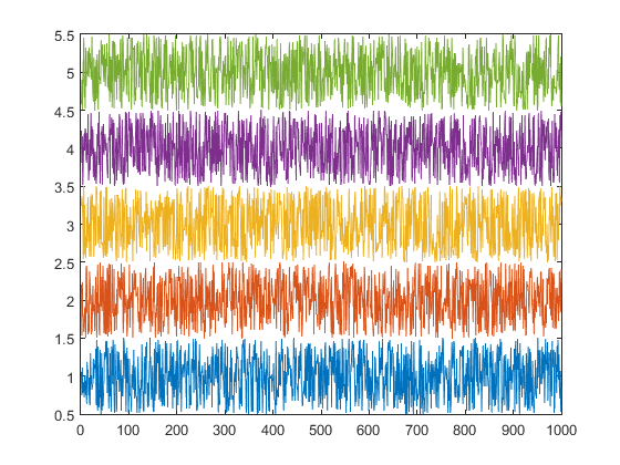
This is very useful for many operations that one would like to perform column-wise or row-wise on an array. For example, if one wants to plot some data with some space between the lines.

x = rand(1000,5)-.5;
plot(fn_add(x,1:5))

fn_normalize normalizes data in specific dimensions by subtracting (or dividing by) the average in those dimensions. In the following example, a 3D data (space x space x time) is first normalized temporally by dividing by an average frame, then by subtracting an average time course.

For an illustration, let us generate a example data, made of a reference image, which is perturbated by some relevant signals specific to some pixels, a non-relevant signal common to all pixels, and additional white noise.

nx = 11; ny = 11; nt = 12;
[x y] = ndgrid(-5:5,-5:5);
t = linspace(0,1,12);
reference = 1+exp(-(x.^2+y.^2)/3^2);
signal1 = 1e-2*[0 0 0 1 1 1 0 0 0 0 0 0];
map1 = zeros(nx,ny); map1(2:5,4:7) = 1;
signal2 = 1e-2*[1 -1 1 -1 1 -1 1 -1 1 -1 1 -1];
map2 = zeros(nx,ny); map2(7:9,7:9) = 1;
relevantsignals = fn_mult(map1,shiftdim(signal1,-1)) ...
    + fn_mult(map2,shiftdim(signal2,-1));
globalsignal = 1e-1*sin(2*pi*t);
globalsignal = shiftdim(globalsignal,-1);
allsignals = fn_add(relevantsignals,globalsignal);
noise = 2e-3*randn(nx,ny,nt);
data = fn_mult(reference,1+allsignals) + noise;

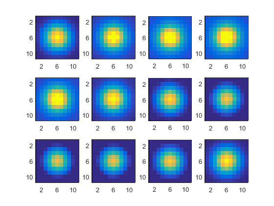
We can only guess the global signal in the raw data.

for k=1:nt, subplot(3,4,k), imagesc(data(:,:,k)',[1 2]), axis image, end

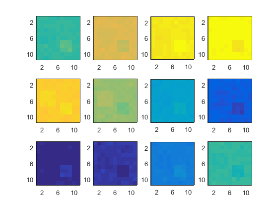
We use fn_normalize to divide by the average frame: the resulting display is still dominated by the global signal.

data = fn_normalize(data,3,'/');
for k=1:nt, subplot(3,4,k), imagesc(data(:,:,k)',[.9 1.1]), axis image, end

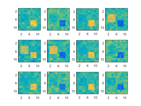
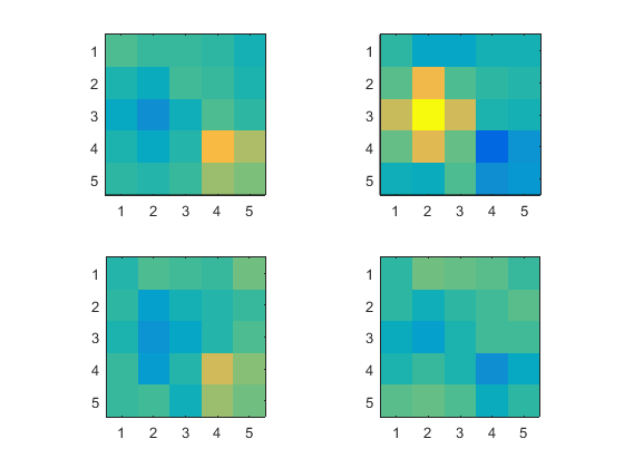
We use fn_normalize to subtract the average time courses: the relevant signals can now be observed.

data = fn_normalize(data,[1 2],'-');
for k=1:nt, subplot(3,4,k), imagesc(data(:,:,k)',[-.015 .015]), axis image, end

Note that the two operations could have been done at once, by doing

data = fn_normalize(data,{3 [1 2]},{'/' '-'});

fn_bin can be used to bin the data above, using spatial bins of size 2x2, and temporal bins of time 3.

databin = fn_bin(data,[2 2 3]);
for k=1:4, subplot(2,2,k), imagesc(databin(:,:,k)',[-.006 .006]), axis image, end

Programming

fn_flags is a convenient function to check which flags are provided to a function through the varargin variable.

Suppose we have a function to which we can pass the flags 'bin', 'txt', 'image' and 'repeat', and the user passed only the flags 'bin' and 'image'.

varargin = {'bin' 'image'};

A quick way to check which flags were passed is:

[dobin dotxt doimage dorepeat] = fn_flags('bin','txt','image','repeat',varargin)

dobin =

     1


dotxt =

     0


doimage =

     1


dorepeat =

     0

fn_switch simplifies the writing of code which would necessit a if or a switch block.

Instead of

if x==0
    y = 0;
else
    y = 1/x;
end

use

y = fn_switch(x==0,0,1/x);

And instead of

switch x
    case 'dog'
        y = 'cat'
    case 'yellow'
        y = 'blue'
    otherwise
        y = 'void'
end

use

y = fn_switch(x,'dog','cat','yellow','blue','void');

Graphic functions

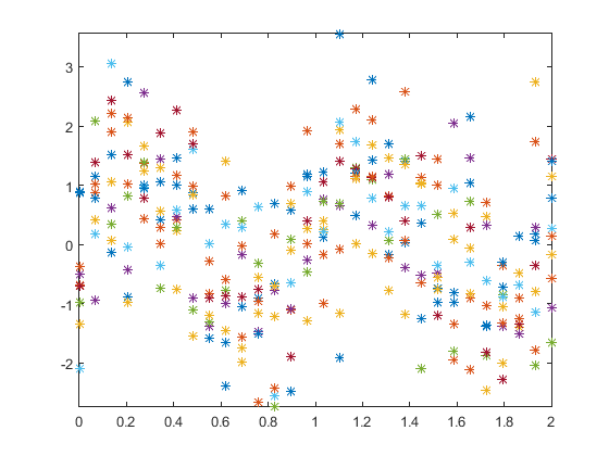
fn_errorbar plots functions +/- error level

Let us create some data: 10 noisy versions of the same sinusoide.

clf
nt = 30;
nexp = 10;
t = linspace(0,2,nt);
signal = sin(2*pi*t)';
data = fn_add(signal,randn(nt,nexp));
plot(t,data,'*'), axis tight

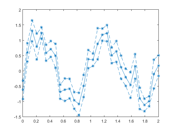
We can compute the average time course and the estimated error, and display the estimation result with fn_errorbar.

avg = mean(data,2);
err = std(data,0,2)/sqrt(nexp);
fn_errorbar(t,avg,err,'*')

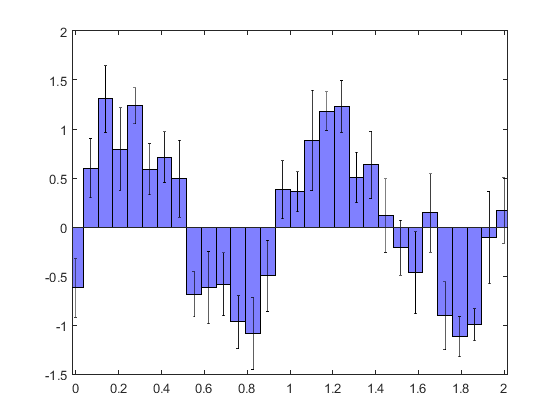
Note that fn_errorbar can also compute by himself average and standard error, and offers also the 'bar' and 'patch' display options.

fn_errorbar(t,data,'bar','facecolor',[.5 .5 1])

GUI basic tools

fn_buttonmotion executes a task while the mouse is moving, and until the mouse button is released. The example below displays the pointer position in the figure whenever the mouse is pressed and moved.

figure(1), clf
ht = uicontrol('style','text','backgroundcolor','y');
fun = @()set(ht,'string',num2str(get(1,'CurrentPoint')));
set(1,'buttondownfcn',@(u,e)fn_buttonmotion(fun,'doup'))

(execute)

GUI elaborate tools

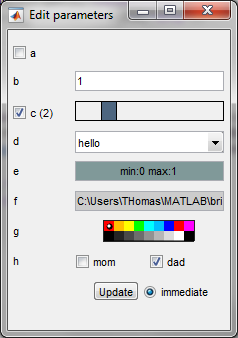
fn_control transforms a structure s into a fn_control object X based on s and displays controls in a figure or a uipanel. The control actions are to modify the values in X, and inversely, modifying the values in X changes the control displays. Below is a simple usage example. See fn_movie function for a more elaborate usage.

s = struct('a',false,'b',1,'c',2,'d','hello','e',[0 1],'f',pwd,'g','red','h',[0 1]);
spec = struct('c','xslider 0 10 1','d',{{'hello','yo'}},'e','clip','f','dir','g','color','h',{{'multcheck' 'mom' 'dad'}});
myfun = @disp;
fn_control(s,spec,myfun);

(execute)

GUI programs

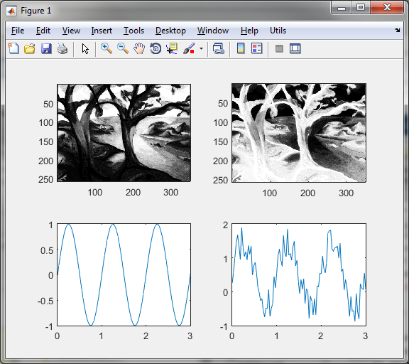
fn_imvalue, when executed, automatically links together the image and plot displays (existing one, and any one which will be created later), so that one can zoom in, zoom out, select a point in an image and get its value, and this simultaneously in all the axes containing data of the same dimensions. Try the following lines to get an idea.

fn_imvalue image
figure(1), clf, colormap gray
load trees
subplot(221), imagesc(X)
subplot(222), imagesc(-X)
nt = 100;
t = linspace(0,3,nt);
signal = sin(2*pi*t);
subplot(223), plot(t,signal)
subplot(224), plot(t,signal+rand(1,nt))

(execute)

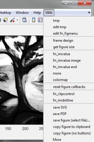
fn_figmenu creates a new menu in all figures opened, and in all figures which are going to be created later, which offers a set of actions. Try it!

Miscellaneous

fn_email allows to send emails from Matlab without leaving the Command window. It can send figures (saved in both the PNG and EPS formats), m-files or any file located on the path, and of course text. Just try it!

Published with MATLAB® R2015a